Characterizing the evolution of entorhinal cortex in AD patients

Projects | 2019 | Links:

A modified geodesic model for characterizing a long term evolution of subcortical structures such as entorhinal cortex (ERC)

Abstract

Early anatomic change of the entorhinal cortex (ERC) provides us with information about the potential pathological structural deformation due to the Alzheimer’s Disease. To better understand the personalized pathological change in ERC, we first describe a mean deformation trend of ERC over a long period of time as a prior distribution using geodesic regression. Then we modify the basic geodesic regression model to investigate the personalized deviation from the mean deformation trend. The result shows that more atrophy and thickness reduction happen in the ERC in subjects who have mild cognitive impairment than normal population.

Background

The localized anatomic changes in brain associated with the Alzheimer’s Disease (AD) is considered as an indirect measurement of neural damage[1]. In particular, the entorhinal cortex is demonstrated a subcortical structure whose atrophy and thickness show a significant relationship with early pathological deformation in patients developing AD[2]. To investigate the deformation of entorhinal cortex at a preclinical stage, we focus on the patients who have mild cognitive impairment (MCI) then progressing to AD.

Computational anatomy provides a possible approach to compute the deformation quantitatively. Characterization of atrophy in entorhinal cortex can be reflected by smooth longitudinal mapping, which is also known as diffeomorphism. Diffeomorphometry describes the correspondence and changes between time-varying templates under the premise of smoothness[2]. In this project, we fit in the time-varying entorhinal cortex templates using the method of diffeomorphometry.

Problems

People have been trying for years to find out what is happening in our brain due to aging or due to some specific diseases on the top of aging, such as AD[3]. Linear models used to describe the changes in longitudinal brain templates appear to perform well in a short period of time. However, long-term deformation is considered non-linear and anatomically localized.

Characterizing the mean evolution of brains at a statistic level can be very valuable for the understanding of outliers which may be caused by diseases. Thus, to draw a mean deformation trend of normal brains and observing the deviation of MCI population will help us identify the pathological changes associated with AD at an early stage. In our project, we are trying to characterize the mean evolution of normal ERC as a prior distribution and find out personalized deviation from the mean to investigate pathological AD-related structural changes.

Methods

Overview

We describe the deformation of each subject’s time-varying ERC templates as a continuous smooth trajectory passing from the baseline through each follow up templates. Our approach to quantify the deformation is to measure the velocity of the trajectory at each moment. The velocity field generated by a single subject is expected to be 4-dimensional in terms of time and space to adapt to high-dimensional time and regional shape variability. Statistically, we average all subject-dependent velocity fields of normal population according to their birthdays to obtain the mean deformation trend associated with aging. Under the influence of the mean trend, we further identify the deviation of MCI subjects from the mean trend to observe the structural change due to pathology.

Subjects

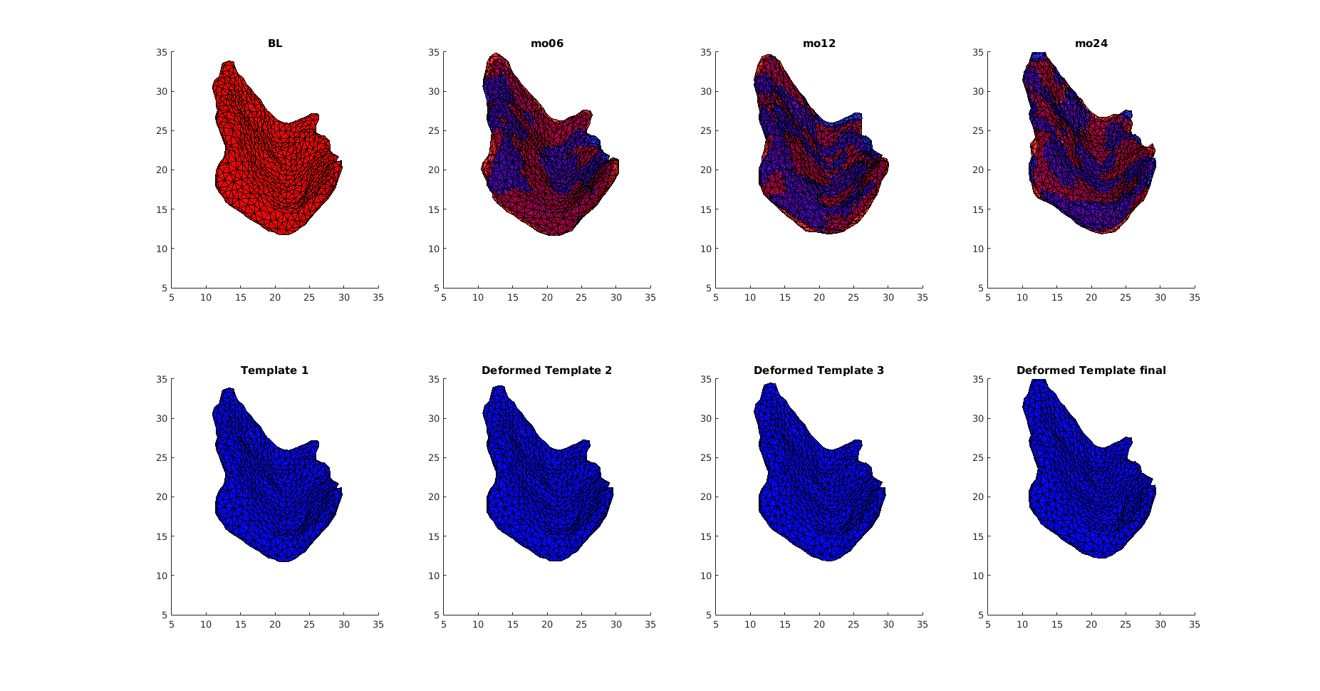
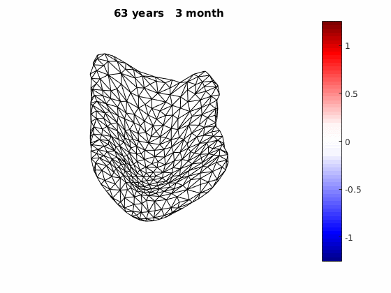
The Alzheimer’s Disease Neuroimaging Initiative(adni.loni.usc.edu) has provided us with a bunch of longitudinal MRI brain scans of normal/control subjects and MCI/non-control subjects. Subjects included in this dataset were in their 60s to 70s when scanned. Most of their scans were acquired at 6, 12, and 24 months after the baseline. People have segmented the scans manually to get triangulated entorhinal cortex templates of subjects in each group. Templates have already been rigidly aligned to its baseline then all onto the baseline of one single subject. An example set of templates of one subject is shown in Fig.1

Fig.1. Orignial segmented ERC of one patient acquired at baseline(left) and 6, 12, 24(right) months after

Rigid registration

We only want to measure the non-rigid deformation of the ERC, and thus we apply rigid registration to eliminate the rigid part as much as possible. Each patient’s templates were all previously registered to their baseline and all patients’ baselines were aligned with a specific baseline. On the top of that, we also optimize some rigid motion parameters including translation and rotation while computing the geodesic trajectories. Since the points in the templates have no one-to-one correspondence over time, our registration is based on current matching algorithm[4].

Geodesic Regression

Even though the consistency of the segmentation can be assured, we cannot avoid the noise while segmenting. Therefore, the segmented templates are not exactly accurate. The problem is that the deformation of the time-varying templates may not be smooth as what it should be in the reality, which means, the shape of the templates may change in opposite directions over time.

To deal with this problem, we use geodesic regression [5] to fit in the time-varying ERC templates. What geodesic regression does is to deform a template over time to match the target templates at each moment but still make sure the deformation remains smooth. Mathematically, we give each vertex of the triangulated ECR templates an initial velocity and have it shot with time. Then a smoothing filter is applied to assure the smoothness of the deformation. And finally, we optimize the initial velocity using machine learning based on declining the difference energy and regularization loss between the deformed templates and the target templates with current matching algorithm [4]. How a deformed template is changing over time to match the original scans is shown in Fig.2 .

Fig.2. Deformed templates(green) shooting towards targets(red).

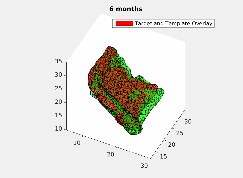
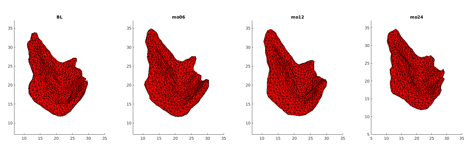
Then we have a trajectory describing a patient’s ERC over two years. In order to test the accuracy of the trajectory, we sample it at the time when the original scans were acquired and do comparasion as shown in Fig.3.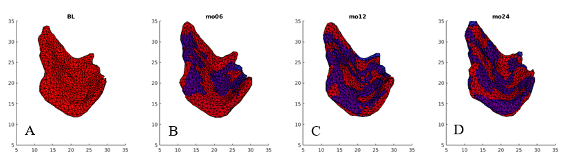

Fig.3. Longitudinal entorhinal cortex target templates(red) and deformed templates overlay(blue) using geodesic regression. (A) Baseline scan. (B-D) Target templates and deformed templates in 6 months, 12 months and 24 moths after the baseline scan respectively.

Average Velocity fields

Our approach to average the velocity fields is a spatiotemporal statistical processing of the longitudinal data [6]. At each time point, we measure the velocity of each subject i on every vertex and then map the velocity field into a standardized dense grid, in which j stands for every grid point. Our time synchronization is based on the subjects’ birthdays.

$$\overline u_j (t) = avg(\sum_{i}{u_{ij}(t)})$$

The mean time-varying velocity field is generated by average each subject i ’s velocity at identical ages and corresponding grid point j. This 4-dimensional velocity field is the quantified mean deformation trend we obtain.

We can do something fun once we get our long-term deformation trand, that is, to flow an estimated template over AD and normal deformation trends respectively:

Fig.4. An estimated template flowing over two different deformation trends. Left: Normal trend Right: AD trend

The normal component of the log determinants of Jocobian matrice were plotted on the surface where blue means shrinkage in thickness (log determinant<0) while red means expansion (log determinant>0). Not surprisingly, the one floated over AD deformation trend appears to have more shrinkage.

Individual deviation

We implement a similar optimization as abovementioned geodesic regression but modify it by regarding the mean deformation trend as a background flow. In the kinetic computation, we initialize the velocity with the mean control flow velocity at corresponding time. Then we add a residual to the initial velocity, which when optimized can produce a reasonable trajectory that still hits all the targets. The optimized residual we obtain here reflects the deviation of the control subjects and MCI subjects from the mean control flow respectively.

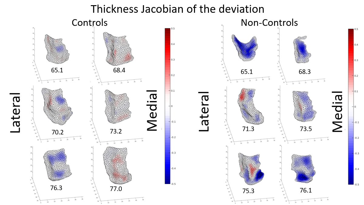
The deviation is measured in terms of atrophy and thickness. We compute the log determinants of Jacobian matrix corresponding to the baseline. The log Jacobian determinants indexed to the template surface on vertices is for analyzing the local structural deviation of the ERC. The log Jacobian of the deviation plotted on each vertex in term of surface atrophy and thickness is shown in Fig.5 , in which blue means log Jacobian is below zero (atrophy in respect with mean flow) , while red means log Jacobian is above zero (expansion in respect with mean flow).

Fig.5. Log thickness Jacobian of the deviation from mean control flow on each vertex plotted on the surface of subjects’ templates

Deviation quantification

Statistic tests

---

Conclusion

Building up a library displaying the evolution of our brain has always been dreamed about. In this project, we compute the deformation of the entorhinal cortex of normal subjects in a relatively long period of time using computational anatomy and geodesic regression. Also, we modify the geodesic regression process to figure out the deviation of MCI subjects from the mean flow. It turns out that there’re more atrophy and thickness reduction in MCI subjects’ entorhinal cortices. This difference of structural changes can help us better understand the pathological deformation due to AD on the top of aging.

The model used in the project can also be extended to other brain structures to obtain a valuable description on the evolution of our brains, which can be also known as prior distribution of brain deformation.

Reference

[1] Atiya M., Hyman B.T., Albert M.S., Killiany R. Structural magnetic resonance imaging in established and prodromal Alzheimer disease: a review. Alzheimer Dis Assoc Disord. 2003;17:177–195.
[2] Miller, M. I. , Younes, L. , Ratnanather, J. T. , Brown, T. , Trinh, H. , & Postell, E. , et al. (2013). The diffeomorphometry of temporal lobe structures in preclinical alzheimer"s disease. NeuroImage: Clinical, 3, 352-360.
[3] Lorenzi M, Pennec X, Frisoni G B, et al. Disentangling normal aging from Alzheimer’s disease in structural magnetic resonance images.[J]. Neurobiology of Aging, 2015, 36:S42-S52.
[4] Vaillant M, Glaunès J. Surface Matching via Currents[C] Biennial International Conference on Information Processing in Medical Imaging. 2005.
[5] Fletcher P T . Geodesic Regression and the Theory of Least Squares on Riemannian Manifolds[J]. International Journal of Computer Vision, 2013, 105(2):171-185.
[6] Durrleman S, Pennec X, Trouvé A, et al. Toward a comprehensive framework for the spatiotemporal statistical analysis of longitudinal shape data.[J]. International Journal of Computer Vision, 2013, 103(1):22-59.