MRI Notes: FID artifact in SE sequence?
in My Blog on Radiology
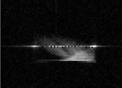
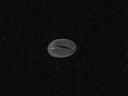
When I was doing the MRI spin-echo experiment, I found there was an obvious fine line at the middle of the final image we obtained (as shown above). Trust me, I was trying to image a peanut, maybe with some water at the bottom(the bright part). Yes, it is a peanut, imaged by an old weird MRI scanner with horribly inhomogeneous 0.5T magnetic field. However, even though the scanner was old, it should never be blamed for the fine line in the middle. Let’s find out the true origin of this artifact and exonerate the scanner.
Spin-echo Sequence
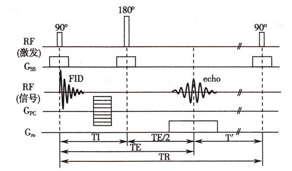
To start with, let’s have a brief look at what spin-echo(SE) sequence is.
SE sequence is a widely used MRI sequence in clinical application. The main feature of it is that it uses a 180° RF impulse to flip the transverse component of the magnetization to another side and thus refocus the phase after dispersion. In other word, the 180° impulse acts like a starting gun which requires all protons to turn around halfway. Therefore, those fast runners who used to lead now have to chase for those slow runners for the same distance.
Advantages of SE sequence
Theoretically, it can eliminate the extra phase dispersion due to magnetic field’s inhomogenity, which means, the time constant of the echo decay would be T2 instead of T2* in gradient-rephase sequence. Thus, the signal intensity will be higher during signal acquisition.
Imperfection of the 180° impulse
Then what is wrong with the SE sequnce now that it is so useful?
We know that it is impratical to perform an infinitely long RF impulse. We cut it off into finite time and sacrifice its frequncy profile correspondingly. This is how the real frequency spectrum looks like:
Gonna be an image here
Therefore, we can see not all protons in the selected slice can be flipped exactly 180°, while those who are filpped bigger or smaller than 180°, will remain a transverse component on XOY plane. And eventually, this residual will induce an FID signal into signal acquisition.
From FID signal to the fine line
Then, what does the FID signal have to do with the fine line? Let’s deduce their relationship step by step on MATLAB.
Model
To make things easier, let’s assume we are now imaging a homogeneous object in the middle of the FOV. It is only a plane so there is no slice selection. Every while pixel would generate its own FID signal, but notice that what we are doing is to produce the artifact of FID signal, not reconstructing this image.

Setting the parameters
First, let’s set some parameters of the object we are imaging and the image we are expecting to acquire.
clear all; clc;

% Object Parameters
gamma = 42.58; % MHz/T
T2 = 300; % ms
T2_star = 15; % ms
length = 180; % mm
width = 180; % mm

% Image parameters
dx = 1.5; % mm  x_resolution
dy = 1.5; % mm  y_resolution
Nx = 256; % 256 x 256 pixels
Ny = 256;
FOVx = Nx * dx; % mm
FOVy = Ny * dy; % mm

% Sequence parameters
ACQ = 12.8; % ms signal acquisition time
BW = 1/ (ACQ/Nx); % kHz
t = 0: ACQ/Nx: (ACQ-ACQ/Nx);
Gx = BW * 1000 / gamma/ FOVx; % mT/m
FID signal acquisition
We are going to generate a FID signal map of Nx * Ny * Time, where the first two dimensions stands for every pixel while the third dimension stands for time ( we sample Nx points in the time domain).
Notice that our phase encoding is added before the 180° impulse, therefore, the FID signal does not undergo phase encoding . However, during the signal acquisition, the FID signal has been frequency encoded.
X = width/dy;
Y = length/dx;
w = gamma*Gx/1000*(-X/2:1:(X/2-1));% kHz frequency encoded percession speed in X-direction
w_object = repmat(w,Y,1); % kHz percession speed of each pixel in the object
phase_map = repmat(w_object,1,1,Nx).*permute(repmat(t,Y,1,X),[1,3,2]); % the third dimension is the phase of each time point
FID_map = cos(2*pi*phase_map).*exp(-permute(repmat(t,Y,1,X),[1,3,2])/T2_star); % Nx * Ny *Time FID map with T2* decay
FID_map = padarray(FID_map,[(Ny-Y)/2,(Nx-X)/2,0]);
figure; plot(t,squeeze(FID_map(100,100,:))); % FID signal of one pixel
FID = squeeze(sum(sum(FID_map))); % FID signal in one loop;
figure;plot(t,FID);
figure; plot(1:Nx,fftshift(fft(FID)));
The plotted pictures are as follows:
1) The FID signal of a pixel ![]()
2) The sum of FID signals we acquire 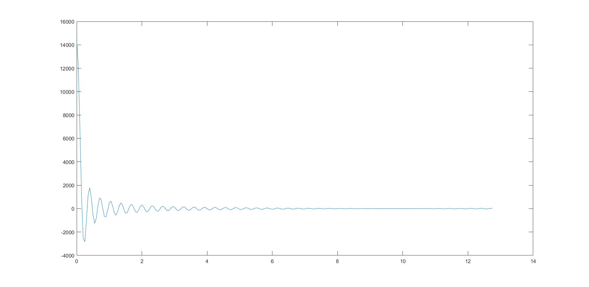
3) 1D Fourier transformation of acquired signal 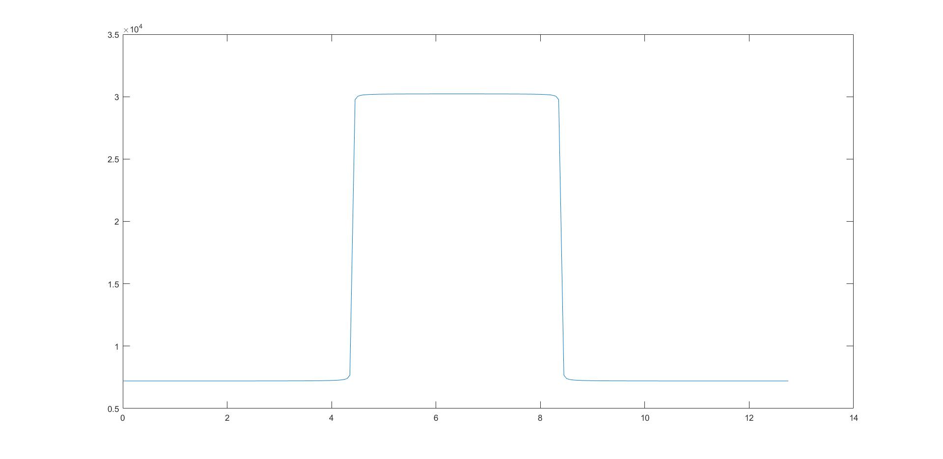
Image reconstruction
OK, now we’ve got the sum of FID signals in one loop, which can fill in one row of the K-space. Since our phase encoding is applied before FID signal’s generation, the FID signal won’t change in each loop. Therefore, we can easily fill in the whole K-space. After 2D FFT, we can see the fine line in the reconstructed image.
K = squeeze(repmat(FID',Ny,1));
figure;
subplot(1,2,1);
imshow(K,[]);
subplot(1,2,2);
imshow(fftshift(fft2(K)),[]);

We also find that the line wasn’t limited in the location of our object, and it also occurs in the dark area with lower magnitude. This is probably because there is a spectrum leakage while we are sampling the FID signal. The specific reason will not be explained in this article.
Remove the artifact
Then, what are we gonna do to remove the artifact? Here, I introduce a method to suppress this fine line artifact in imaging part.
To suppress the impact of FID signal, we cannot let it “freely decay”. So, after it is induced by the 180° impulse, we can apply an extra gradient to disperse the phase of FID. In the meantime, we should also apply an inverse gradient before the 180° impulse to make up for the crusher’s influence on the wanted signal. Theoretically, the bigger the area of the gradient is, the better the effect of the artifact elimination will be.
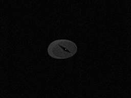
We did another experiment to see how the crusher worked later. Here are the image we obtained without & with the crusher.
Without crusher:
 With crusher:
Conclusion
ALright, as we can see in these two pictures, the fine line has been suppressed by the crusher. This is because the FID signal is dispersed, so that it won’t influence the image too much. However, we can still see a bright spot in the middle of the image. We tried several methods to eliminate this spot but they all didn’t work. I still haven’t found out what induces this DC component. Let’s see if I can figure it out in the future.